JigCell Run Manager User's Manual
The JigCell Run Manager (JCRM) allows a user to define a set of
specifications for simulation runs using a spreadsheet interface.
Each row of the spreadsheet describes the information necessary for a
single simulation run.
While this is not the only way that JCRM can be used, the typical use
is to create an ensemble of simulation runs related to a specific
biomolecular reaction model, where each run differs from the others in
only minor ways.
Thus, JCRM provides support for defining simulation runs in terms of
minor differences from other simulation runs, with the potential of
building up a hierarchy of such differences.
This makes it easy to define small parameter changes that affect many
simulation runs.
JCRM serves two chief purposes.
The first is to let users provide the specifications needed to run
a simulation that matches a particular experiment.
The second is to let users organize related simulation runs,
and then run and view the results of either the entire ensemble or of
a single simulation.
1 - Overview
Cell cycle modeling often involves defining a model, which captures
the differences among potentially hundreds of mutations of the wild
type organism.
This is represented by a simulation run for each such mutation, where
each simulation run differs from others in a small number of
parameters.
JCRM allows users to express a hierarchy of simulation runs that
define the minor differences between runs.
That is, one run might be identical to a base run, except for changes
to a few parameters or initial conditions.
Hierarchies can be built up, whereby a given simulation inherits the
differences from the wild type from one or more other runs.
Developers of sophisticated cell cycle models do not want to
have to edit all such simulation runs (and there could be hundreds of
these) when they wish to change one or two parameter values shared by
all such runs.
JCRM's run hierarchies avoid this problem.
JCRM provides a sophisticated mechanism for keeping track of logical
relationships among simulations done on a single model to fit a
variety of experiments and allows the modeler easily to explore the
parameter space of a model over a
complicated set of simulations.

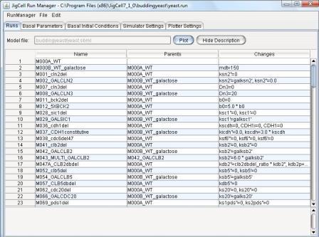
Figure 1. A simulation ensemble for budding yeast cell mutants.
2 - Major Interface Components
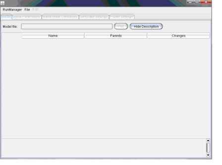
On startup JCRM screen will appear as in Figure 2.
JCRM has two main user interface components: the menubar and the
tab bar.
The tab bar is disabled until a run file has been loaded.

Figure 2. JCRM on start up.
3 - JCRM Menu Bar
The JCRM Menu Bar has three items:
RunManager, File, and Edit.
Only the first two are enabled when there is no run file loaded.
-
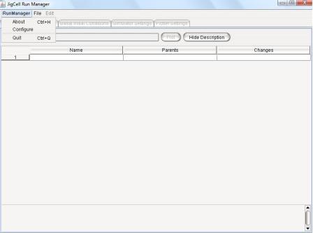
RunManager - This menu gives information about the application,
and allows you to quit the program. See Figure 3.

Figure 3: RunManager Menu
-
About -
Display an information box giving the current JCRM version number
and contact info for the JigCell team.
-
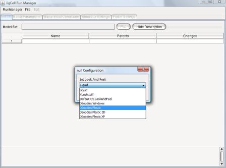
Configure
The Configure option gives the user a chance to change the look and
feel of the program (Figure 4).

Figure 4: RunManager/Configure
-
Quit -
Exits the program.
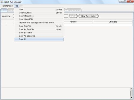
- File: Allows the user to manipulate files.

Figure 5: File Menu
- New - Initiate a new run manager instance with empty
spreadsheets.
- Open Run File - Open a run file (these have a ".run"
extension).
A run file contains a complete specification for an ensemble of
simulation runs.
It contains runs, basal parameters, basal initial conditions,
simulator settings, and plotter settings, as required for a
simulation.
-
Open Model File - Open an SBML file
-
Open Basal File - Open a basal parameter set file (these
have a ".bas" extension).
This defines the "basal" parameters and initial conditions for a
model.
-
Import basal settings from SBML Model - Open a SBML file,
extract the basal parameters, and save them to a basal file.
The related spreadsheets (basal parameters and initial conditions) are
populated from the SBML file.
-
Save Run File - Save the currently active run file.
If the active file has not yet been saved, a Save dialog box will
prompt the user to choose a location and enter a name for the
file.
-
Save As Run File - Also saves the active run file, however,
this will always ask the user for a location and name.
-
Save Basal File - Save the active basal parameter file.
If the active file has not yet been saved, a Save dialog box will
prompt the user to choose a location and enter a name for the
file.
-
Save As Basal File - Also aves the active basal file, however,
this will always ask the user for a location and name.
-
Save All - Gives user an option to save all open files.
-
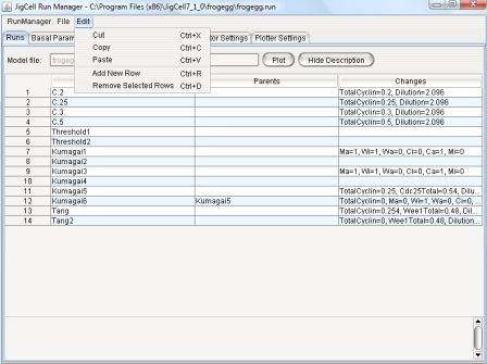
Edit - The edit menu becomes enabled when user opens a file
(model/basal/run) from the File menu.
It provides the ability to edit data in the spreadsheets (Figure 6).

Figure 6: Edit Menu
-
Cut - Remove whatever is currently selected and place it on a
clipboard.
-
Copy - Remove whatever is currently selected and place it on a
clipboard.
-
Paste - Place a copy of the current clipboard contents at
the current cursor location in the spreadsheet.
Contents may not be pasted to different tabs or spreadsheets.
- Add New Row - Add 1 row to the end of the currently
displayed spreadsheet.
-
Remove Selected Rows - Delete the selected rows.
4 - JCRM Spreadsheets
JCRM manages the description and execution of ensembles of simulation
runs using a tabbed spreadsheet interface.
To specify a simulation run, the user must provide a model, a
parameter set, an initial condition set, and a simulator parameter
set.
Each of these is specified using its own tab.
Thus, there are five tabs in the JCRM interface.
These are each described below.
-
4.1 - Runs Spreadsheet
The Runs spreadsheet interface allows the user to define a series
of simulation runs, one run per row.

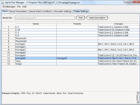
Figure 7: Runs Spreadsheet (showing the frog cell model .run file)
The Runs spreadsheet contains 3 columns.
-
Name - Specifies the name of a run (or experiment)
-
Parents - The 'Parents' column indicates the name of the parent
run(s).
The current experiment will inherit its parameter values and initial
conditions from its parents.
Thus, the parents column defines a hierarchy relationship between
runs.
See 4.1.1 - Parents
Editor for details on how to edit an entry in the Parents column.
-
Changes - The 'Changes' column defines a list of basal
parameters, initial condition, simulator settings, and plotter
settings that have been changed for the current run.
The changes are made using the changes editor, which opens when
clicking on the changes cell for a particular run.
See 4.1.2 - Changes
Editor for details on how to edit an entry in the Changes column.
The Runs spreadsheet also contains these additional interface
elements.
-
The Model File field lists the name of the model file currently
being accessed for basal paramter values.
-
The Description field appears at the bottom of the Run Manager
interface when it is visible.
-
The Hide/Show Description buttons allow the user to hide or
reveal the description field at the bottom of the screen.
-
The Plot button allows the user to execute the simulation
defined by the currently selected row, and displays a plot of the
results.
This feature is handy in checking that all the information for
simulating this particular experiment has been correctly entered.
For instance, Figure 7 shows a Run Manager spreadsheet for simulating
some experiments done on frog cell extracts to characterize the
activation of MPF.
Each row defines a separate experiment.
Rows 1-4 describe four experiments done by Jonathon Moore (Duke
University) on MPF activation in extracts prepared with different
amounts of non-degradable cyclin B (20, 25, 30 and 50 nM).
(Note that this information is presented in the description field).
The parameter sets are derived from the same basal set
(whatever the basal parameter values happen to be), the only
difference being that the parameters/initial conditions "TotalCyclin"
and "Dilution" are set appropriately in each row.
-
4.1.1 - Parents Editor
The 'Parents' editor allows the user to add or change the parents of a
given run.
The current experiment will inherit its parameter values and initial
conditions from its parents.
Thus, the parents column defines a hierarchy relationship between
runs.
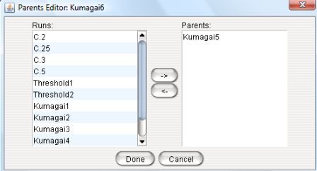
Clicking on the parent cell opens up the Parents Editor for
that run (see Figure 8).

Figure 8: The Parents Editor.
In this editor user gets a list of all the runs (on the left hand side panel) and can select a run as a parent of the curent experiment or
deselect previously selected runs.
-
4.1.2 - Changes Editor
The 'Changes' editor defines a list of basal parameters,
initial condition, simulator settings, and plotter settings that have
been changed for the current run.
The changes are made using the changes editor, which opens when
clicking on the changes cell for a particular run.
The changes for a particular run override the changes inherited by any
parents and propagate to its children.
clicking on the Changes field for a given run opens the Changes
Editor.

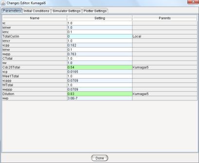
Figure 9: The Changes Editor.
This editor has four spreadsheets - Parameters, Initial Conditions, Simulator Settings and Plotter Settings.
The purpose and structure of each of these spreadsheets are similar to the Run Manager's principal spreadsheets, but they represent the values for the current experiment.
Using these four tabs user can change any parameter/simulation settings and can change the plotter settings or can alter the selection of variables to plot.
If user changes one of the values, that becomes highlighted with sky-blue. The cyan colored values represent the changes done in the parent runs and the other ones are inherited from original run.
-
4.2 - Basal Parameters Spreadsheet
Basal parameter sets are defined initially by the SBML file.
The user may then change any of the basal parameter values by clicking
on the Value cell for any parameter.
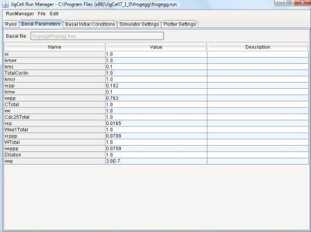
Those values that have been changed by the user are colored in orange.

Figure 10: Basal Parameter Spreadsheet.
The Description field Contains a text description for the
parameter.
The user can edit the contents of this field by clicking on it.
-
4.3 - Basal Initial Conditions Spreadsheet
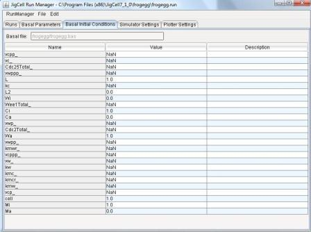
Basal initial conditions defined initially by the SBML file.
n existing model.
The user may then change any of the basal parameter values by clicking
on the Value cell for any parameter.
Those values that have been changed by the user are colored in orange.

Figure 11: Basal Initial Conditions Spreadsheet.
The Description field Contains a text description for the
parameter.
The user can edit the contents of this field by clicking on it.
-
4.4 - Simulator Settings Spreadsheet
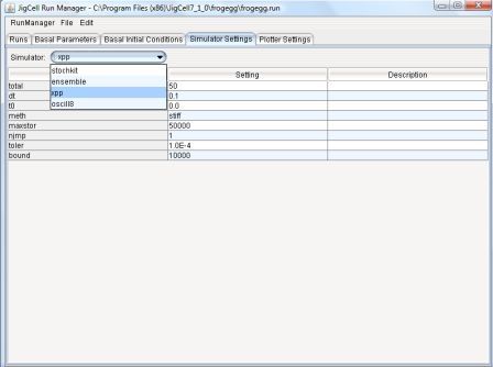
The Simulator Settings spreadsheet allows the user to define
parameters that affect the operations of the simulator.
The Simulator field Allows the user to select from a collection
of available simulators.
Each one has an associated collection of parameter settings,
whose defaults are loaded into the spreadsheet when the simulator is
selected from the menu list.
The user can then change any of these defaults by clicking on the
Setting field.
A comment can be entered into the Description field.
Examples for the XPP simulator (which executes ODE models) are total
time of integration, integration method to use, tolerances, output
interval, etc.
Other simulators can be added easily to the Run Manager configuration.
For example, Gillespie's Stochastic Simulation Algorithm has been privided
via the Stochkit simulator.

Figure 12: Simulator Settings Spreadsheet.
-
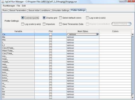
4.5 - Plotter Settings Spreadsheet
The Plotter Settings tab enables the user to specify the variables to
be plotted. The Plotter Settings tab also contains options to customize
the plot by selecting colors, mark styles, whether to connect points,
etc. Alternatively, the user can select to use the default settings
after selecting what variable to plot.

Figure 13: Plotter Settings Spreadsheet.
Near the top of the Plotter spreadsheet are checkboxes that allow the
user to modify plot visual features such as the axis scale (log scale
or linear), and plot line format.
By selecting the "Save TimeSeries Data" user can choose a location to
save time series data as a csv file.
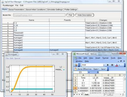
After selecting required variables, the user
can generate a plot (from Runs spreadsheet) and view the csv file for
details (see figure 14).

Figure 14: Plotter Spreadsheet - Plot and Corresponding Data File (.csv File)
The spreadsheet has four columns
-
Variable - the names of the model variables
-
Plot - a checkbox that determines whether the corresponding
variable will be plotted.
-
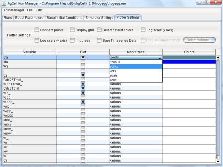
Mark Styes - Defines the symblo used on the line to plot th
ecorresponding variable: various, points, dots, pixels, or no symbol.

Figure 15: Plotter Spreadsheet - Mark Styles
-
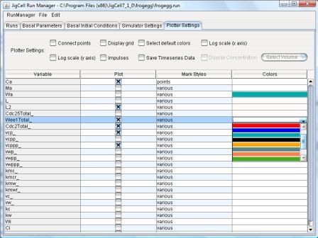
Colors - If the 'Select default colors' checkbox on the top panel
is checked then colors are automatically assigned to plotted
variables.
Alternatively, the Colors column can be used to assign colors to
variables from a color pallet.

Figure 16: Plotter Spreadsheet - Colors
