Example Walkthrough
This walkthrough demonstrates using the Comparator. Users generally follow the same process of entering experimental data, configuring simulations, and configuring comparisons for every job. This example uses the same data as the system tests.
The walkthrough requires the files from the default installation to be in place.
Entering Experimental Data
- Launch the Comparator. By default you'll be in the
Experiment tab. The Experiment tab is a list
of entries that describes a set of laboratory experiments. Each entry in the
Experiment tab consists of four parts:
- Name describes the row and should be unique among all the experiments
- Experiment Value is the experimental observation
- Value Type describes the structure of the experimental observation
- Comment contains some comments from the user
Currently there is just one entry named New.
- Double click on New to edit the name and enter MPF mphase activation L
- Double click in the Experiment Value column for the same row and enter ((2, 0.75),(4,0.51),(8,0.21))
- Double click in the Value Type column for the same row and enter Time-L series
- Double click in the Comment column for the same row and enter Kumagai & Dunphy 1995 Fig 4b
- Check the display against Picture 1
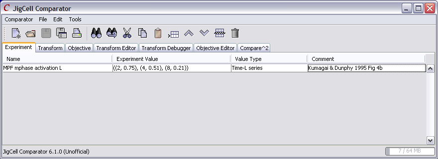
Picture 1
Configuring a Simulation
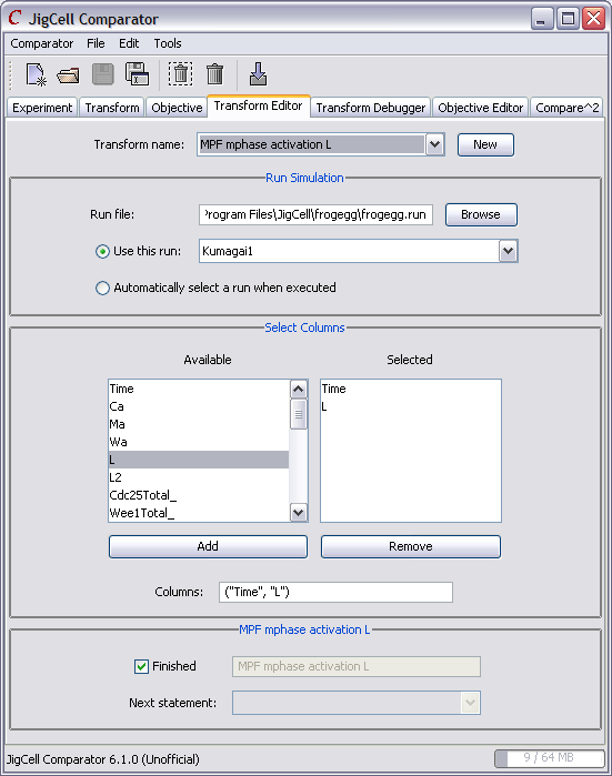
- Switch to the Transform Editor tab. The transform editor tab describes a procedure for performing a simulation. Each procedure consists of a series of steps running from top to bottom.
- Click on the New button and name the transform MPF mphase activation. The dialog box that appears for entering the name also allows you to select from the names of experiments in a dropdown.
- From the Next Statement box, select Run Simulation
- Click on the Browse button in the transform and select frogegg.run from the frogegg directory
- Select Use this run and choose Kumagai1 from the Run box in the transform
- From the Next Statement box, select Select Columns
- Double click on Time and L to select those columns
- Click on the Finished box to remind yourself that you've completed all of the steps for this transform. This completes the description of a procedure that loads the run file froggegg.run, executes the run named Kumagai1, and pulls the Time and L columns of the resulting output into a list of ordered pairs.
- Check the display against Picture 2
- Switch to the Model tab
- In the Transform column for the experiment, select MPF mphase activation. This associates the procedure we've defined with the experimental data.
- Use Run/Run in the menu. If everything worked, the procedure we've defined will be executed and the result will appear in the Transform Value column.
- Check the display against Picture 3
Picture 2
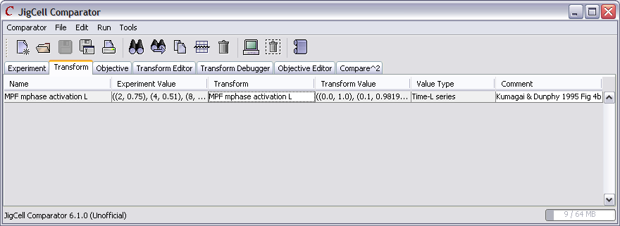
Picture 3
Configuring a Comparison
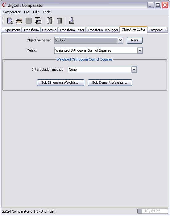
- Switch to the Objective Editor tab. The objective editor tab describes a procedure for performing a comparison.
- Click on the New button and name the objective function WOSS
- From the Metric box, select Weighted Orthogonal Sum of Squares
- From the Interploation method box, select None. This describes a procedure that uses weighted orthogonal sum of squares with no interpolation between model points and leaves the weights with their default values.
- Check the display against Picture 4
- Switch to the Objective tab
- In the Objective column for the experiment, select WOSS. This associates the procedure we've defined with the experimental data.
- In the Criterion column for the same row, select <=
- Double click in the Acceptable column for the same row and
enter 0.005. The Acceptable column is an easy way
of telling the state of a comparison.
- If the entry is white, the value is acceptable
- If the entry is orange, no comparison has been done
- If the entry is red, the value is not acceptable
- Use Run/Run in the menu. If everything worked, the procedure we've defined will be executed and the result will appear in the Objective Result column.
- Check the display against Picture 5
- Try right clicking in the experiment row and selecting Plot to bring up a plot
Picture 4
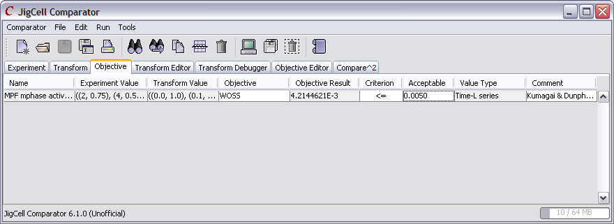
Picture 5
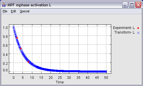
Plot of the experimental results