Frog Egg Extract Model, Use Case, and Walkthrough
[Note: Most figures on this page can be clicked on to open a larger version.]
This page presents a basic use case for the type of biological pathway modeling done in the Tyson lab, and supported by the JigCell software. This use case describes the process by which a researcher initially devises a basic model, and uses software to help refine that model. As part of this use case, the model itself is developed and described in various forms, from initial wiring diagram to initial SBML file to a model verified to match the available experimental data. In addition to this use case, we provide a companion walkthrough whose purpose is to illustrate how the JigCell software is used.
The model developed in this use case is based on the biochemistry of M-phase promoting factor (MPF) in Xenopus oocyte extracts (frog egg extract). It is a simpler model based on an earlier work by Marlovits, Tyson, Novák, and Tyson (1998). This model contains five differential equations, eighteen parameters, and eight initial conditions. Click here for a more complete description of the organism being modeled and what is hyphothesized about the biochemical interactions taking place that lead to the actual reactions shown below.
Once the modeler has decided what process in an organism to model, the next step is to catalog what is currently know about the relevent quantitative and qualitive behavior of the process. In particular, the modeler will find in the literature various pieces of information about the process as exhibited by various mutants in experimental conditions. The reported results of these experiments will include such things as the concentration of various chemical species over time, and perhaps the qualitative outcome such as whether the organism was able to reproduce if the cell cycle is being modeled. Collectively, this information is referred to as experimental data. The experimental data are used first by the modeler to gain insight into the details physiological process being modeled, as in exactly what chemical reactions are taking place. Once a model has been created, the simulation results from the model will eventually be compared against the experimental data to see how "good" the model is.
Click here for a detailed description of the experimental data used to generate and then to validate the frog egg extract model.
The next step in creating a model is to sketch out the relationships between the active chemical species in terms of the reactions that are hypothesized to be taking place. Since the species are typically involved in multiple interacting reactions, the result is network of reactions, and the resulting diagram is referred to as a reaction network or a wiring diagram.
Typically, a modeler will begin by hand sketching the diagram onto a piece of paper. If the modeler has spent a lot of time developing the wiring diagram, he or she might enter it into a CAD program for wider dissemination such as in a publication. Note that this is separate from entering the diagram into a program whose purpose is to support the creation and testing of models (such as JigCell). Click here for a discussion on the pros and cons of various paradigms for model building software interfaces.
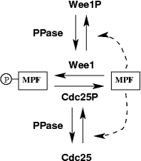
Figure 1. Wiring diagram for the frog egg extract model.
Unfortunately, the wiring diagram provides only a qualitative description of how the chemical species interact. Once the modeler has an idea of what the reactions are and how they interact, the next step is to define the model precisely in terms of a series of reaction equations. At this stage, a reaction equation should include not only the species involved and the direction of the interaction, but also a rate law to quantitatively define exactly how the reaction is taking place. Here is how the frog egg extract model would look in the JigCell Model Builder.
)
Figure 2. The equations for the frog egg extract model.
This model has three parts. Lines 1-4 define rate laws, to be used in the computations for reactions defined later. Lines 5-12 define the reactions, which map to four differential equations (one reaction in each direction). Lines 13-29 define the various chemical species involved. To be complete (and simulatable), values must be provided for all of these species. Some of these values are constants that partly define the organism or some variant of the organism (a mutant). These might be known by the modeler in advance. Others are values that the modeler must determine in order to "fit" the phenomenological data that the model is designed to match. These are called "parameters". The modeler can either guess at these values, or can use parameter estimation software to determine the best values. Either way, some value must be set before the simulation can be run. Other species values can change over time, but need an initial value for the start of the simulation (initial conditions). The modeler enters all of this information into the model builder.
)
Figure 3. Frog egg model parameters.
)
Figure 4. Frog egg model initial conditions.
Click here to see the actual SBML file.
Once the reference or "wild type" organism is defined by the model, the modeler will typically need to run simulations to see if the outcomes are as expected. For our modeling, there is usually information related to a series of mutations for the oganism, which express themselves in modeling terms as fixed values for various model parameters. The idea is that these mutants are testing variations on the model that help to verify that all the pieces are correct. The JigCell Run Manager lets the user specify a set (ensemble) of simulations to model the various mutations. Each line in the Run Manager spreadsheet inferface defines one simulation run.
)
Figure 5. An ensemble of runs for the Frog Egg extract model, as defined in the JigCell Run Manager.
The ensemble above defines fourteen separate simulation runs.
Once the model is completely specified (including reactions, rate laws, parameters, initial values, etc. for the wild type and all the mutants), the user will typically want to run simulations to test how well the model matches expectations. The simplest thing that can be done is to run a single simulation on a single variant of the organism. For the frog egg model, the result is a time series for various chemical concentrations. This time series can be plotted.
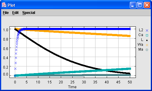
Figure 6. A time series plot for one simulation run.
If the model appears "reasonable" to the modeler for runs on individual mutants, the modeler will soon want a way to guage the performance of the overall model in terms of its ability to match the experimental data for the entire ensemble of mutants. In JigCell, this is done using the comparator.
)
Figure 7. The first step is to enter the experimental data.
To do a comparison, the user must define the relationships between the experimental data and the simulation output, including the definition of a "good match". Once the simuations are executed, those runs not meeting the criteria are shown in red.
)
Figure 8. The results of a comparison.
After studying the feedback from the comparator, the user might then make changes to the various parameter values. After running the ensemble again, the user will have a collection of new results. A tool like Compare2 will permit the user to compare the various models against each other.
)
Figure 9. Using Compare2 to compare two models.
At some point, the modeler will be sufficiently confident in the model such that he or she will want to know what is the best that this particular set of reaction equations can achieve. That is, for this given set of equations, what parameter value settings will yield the "best" result? Automated parameter estimation attempts to answer this question.
Once the parameter estimator has returned the best possible values for this set of reaction equations, the next step will be for the modeler to use what he or she has learned so far to create a new model.