Generic Model of Eukaryotic Cell Cycle Control: Building the Model
The behavior of a regulatory network with interacting feedback loops is hard to understand by intuition alone. Mathematical modeling provides a rigorous and reliable tool for analyzing such complex systems. JigCell was developed to provide a problem solving environment that supports modelling efforts as shown here for the generic cell cycle model .
Building the Model
The JigCell Model Builder helps a modeler to convert
the wiring diagram into an exact mathematical formulation.
It outputs the final model in SBML and .ode formats.
It detects conservation relationships among components of the network.
Here is how the generic cell cycle control model looks like in the
Model Builder.

Fig. 2. Reactions in the generic model.
Reactions are entered into the model builder as follows. When the JigCell Model Builder is opened, on its left panel, there are seven tabs (each is a spreadsheet) marked as Model, Compartments, Parameters, Species, Consevation Relations, Events, and Differential Equations, respectively.
Clicking on the Model tab will open the spreadsheet where the reaction mechanisms are defined. For example, in Fig. 2, Row #8 describes how CycB synthesis is controlled. Since its rate of synthesis (Vsb) is a function of the transcription factor TFB (not a function of CycB directly), the reaction type is chosen as 'Mass_Action_0'. (The behavior of such reactions is defined in Row #3.) The parameter name for this 'Mass_Action_0' reaction, k1, is given as 'Vsb', which is defined later as a species on Row #47. The transcription factor TFB, which affects the synthesis rate, is defined in Row #46 as a species, and its value is evaluated as a GK function. The formula for the GK function is defined in Row #1 and #2.
Similarly, Row #9 describes how CycB is degraded. The reaction type is chosen as 'Mass_Action_1', since the degradation is a first order reaction, depending on the concentration of CycB. But the rate of CycB degradation (Vdb) is not a constant, rather it is proportional to the concentration of two cofactors of APC, Cdh1 and Cdc20, as defined in row #48.
Rows #37 and #38 describe how Cdh1 and Cdh1i are inter-converted between active and inactive forms. Similarly, Rows #44 and #45 describe the inter-conversion between APC and APCP. Since there is no synthesis and degradation, the Model Builder will detect such conservation relationships and will allow the user to assign one as a dependent variable of the other, as shown in Fig. 3 for the Conservation Relations spreadsheet.
The Events spreadsheet allows the user to define conditions for a
specific event to occur in the model.
For example, in modeling the cell division cycle, we assume that
mitosis and cell division occur when the activity of MPF drops
below a critical value KEZ.
When that condition is met, cell mass is divided by two,
half is given to the mother and half to the daughter, as shown in Fig. 3.
Note that the symbol '< 0' means that this condition will be met and the
event will be carried out only when MPF is larger than KEZ at the
previous time step, and it becomes smaller than KEZ at this time step.
The symbol can also be '> 0', which means the condtion is satisfied if
MPF is increasing and reaches the value KEZ from below;
whereas the symbol '= 0' means the condition is satisfied if MPF
reaches the value KEZ from either direction.
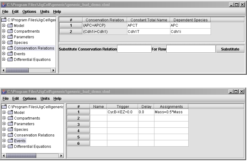
Fig. 3. Conservation Relations and Events spreadsheets.
The names of all parameters that appear in the definitions of Vsb, Vdb, etc,
(marked as Parameters in the last column of the
Model spreadsheet) will appear automatically in the
Parameters spreadsheet, where the values are entered (Fig. 4).
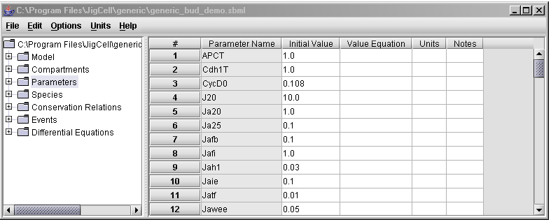
Fig. 4. Parameter values are specified in the Parameters spreadsheet.
The names of varibles and species that appear in the definitions of reactions (2nd column in the Model spreadsheet) will automatically appear in the Species spreadsheet, where the initial conditions for the variables are entered (Fig. 5). Notice that in Fig. 5, values are not needed for any species (e.g. CycBT), since they are calculated by the simulator during each run. Note also in this figure, in the Compartments column, the user can assign the variables to different compartments in the cell, which are defined in the Compartments spreadsheet as shown in Fig. 6.
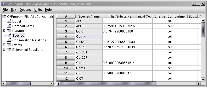
Fig. 5. Initial conditions are descibed in the Species spreadsheet.
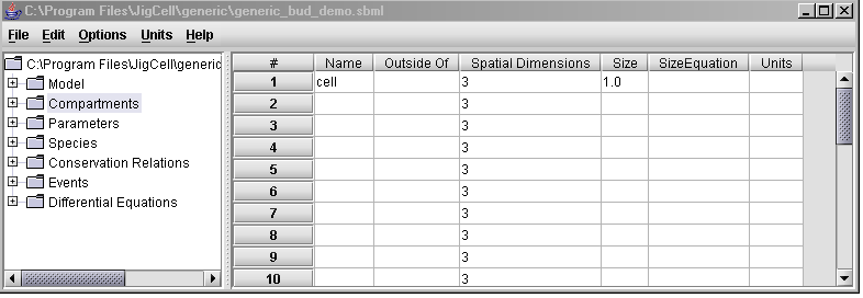
Fig. 6. The cellular compartments are defined in the Compartments spreadsheet.
The Model Builder can display the differential equation for each variable, as shown in Fig. 7.
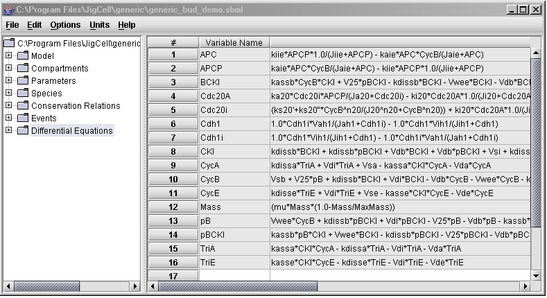
Fig. 7. The Differential Equations spreadsheet.
The Model Builder saves the model equations in SBML format by default. It can also output it as an ode file (used by XPP).
- Click to see the SBML file for the the generic model,
- Click to see the ode file with parameters for budding yeast.
The program sbmltoode.bat will convert an SBML file to an ODE file for use with XPP. To use this program,
- Open a DOS command window.
- Change directory to your JigCell installation root directory.
- Invoke the program with the name of the source SBML file and the name of the target ODE file, as: sbmltoode source.sbml target.ode